Use these 6 Window Functions to power up your PySpark queries, a comprehensive guide
Introduction
Most of the time we use the SQL module in Spark. We create DataFrames with the DataFrame APIs which contain different optimizers that help support the processing of data with a wide range of data sources and algorithms for Big Data workloads.
In SQL, we have a particular type of operation called a Window Function. This operation calculates a function on a subset of rows based on the current row. For each row, a frame window is determined. On this frame, a calculation is made based on the rows in this frame. For every row, the calculation returns a value.
Because Spark uses a SQL module, we also have Window Functions at our disposal. When we combine the power of DataFrames with Window Functions, we can create some unique optimized calculations!
In this article, we'll demonstrate the six most used Window Functions to power up your PySpark queries!
Outline
Window functions can be divided into three category families. We will break down this article into these families and demonstrate real-world examples with detailed explanations.
If you want straight to the code, go to my GitHub repository → 6-window-functions-with-pyspark
Aggregate Functions
The first category of Window Functions are aggregate functions. These Aggregate Window Functions belong to a family that is identical to GROUP BY aggregates.
They operate on a set of values based on the values in the window frame and return a value.
Window aggregate includes the following functions:
- AVG() average of values
- SUM() the total sum of values
- MAX() maximum of the total values
- MIN() minimum of total values
- COUNT() the total number of values
With the help of these functions, you can do some powerful queries! Let's start with the first example.
Cumulative SUM
You can easily calculate a cumulative sum(Running total) with window functions. This calculation is used to display the partial sum as it grows with time. You can easily see the trend of total contributions at any point in time.
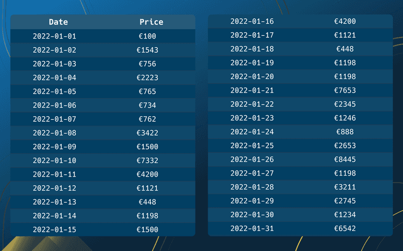
For the two following code examples, we make use of a sales dataset. This dataset contains the total sales on a set of dates.
We load the data into a DataFrame with the use of createDataFrame function and show the first 5 records with df.show(5).
from pyspark.sql import functions as F
from pyspark.sql.window import Window
from datetime import datetime

data = [
    [datetime(2022, 1, 1), 100], [datetime(2022, 1, 2), 1543], [datetime(2022, 1, 3), 756],
    [datetime(2022, 1, 4), 2223], [datetime(2022, 1, 5), 765], [datetime(2022, 1, 6), 734],
    [datetime(2022, 1, 7), 762], [datetime(2022, 1, 8), 3422], [datetime(2022, 1, 9), 1500],
    [datetime(2022, 1, 10), 7332], [datetime(2022, 1, 11), 4200], [datetime(2022, 1, 12), 1121],
    [datetime(2022, 1, 13), 448], [datetime(2022, 1, 14), 1198], [datetime(2022, 1, 15), 1500],
    [datetime(2022, 1, 16), 4200], [datetime(2022, 1, 17), 1121], [datetime(2022, 1, 18), 448],
    [datetime(2022, 1, 19), 1198], [datetime(2022, 1, 20), 1198], [datetime(2022, 1, 21), 7653],
    [datetime(2022, 1, 22), 2345], [datetime(2022, 1, 23), 1246], [datetime(2022, 1, 24), 888],
    [datetime(2022, 1, 25), 2653], [datetime(2022, 1, 26), 8445], [datetime(2022, 1, 27), 1198],
    [datetime(2022, 1, 28), 3211], [datetime(2022, 1, 29), 2745], [datetime(2022, 1, 30), 1234],
    [datetime(2022, 1, 31), 6542],
]
df = spark.createDataFrame(["date", "sales"])
df.show(5)
# +-------------------+-----+
# |               date|sales|
# +-------------------+-----+
# |2022-01-01 00:00:00|  100|
# |2022-01-02 00:00:00| 1543|
# |2022-01-03 00:00:00|  756|
# |2022-01-04 00:00:00| 2223|
# |2022-01-05 00:00:00|  765|
# +-------------------+-----+
# only showing top 5 rows
With our loaded dataset, we can create our first Window Function. We have to call the Window Function within the withColumn statement. In this withColumn statement, we set the name of the column as the first argument. The second argument contains the entire window expression.
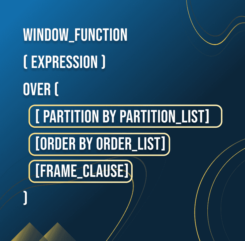
Window Functions follow a structure where a kind of function will be called over a window. In this window a PARTITION BY, ORDER BY, and a FRAME clause can be inserted.
In our example, we are interested in summing up the row consecutively. Therefore we must use the sum Window Function. We know what we mean by consecutively, but it can mean a lot different in Window Functions. literally, it means one after another without interruption. But this doesn’t describe any order.
For our example, ordering the date in ascending order is necessary in order to calculate the cumulative sum correctly. We do this by using the ORDER BY clause.
If we are interested in calculating cumulative sums over different groups, we have to PARTITION BY our data into smaller subsets. For the simplicity of this example, we skip partitioning.
The FRAME clause comes last. This clause is used to determine the bounds of the window. In simple words, it is used to determine the start and end row for each window.
We can begin by defining a Window Function in PySpark now that we are aware of its structure.
.withColumn("cumsum", F.sum("sales").over(Window.partitionBy().orderBy("date")))We select the F.sum Window Function. Then define the Window Frame where the function must be calculated over. This can effortlessly be done by calling the function with the .over() clause. Finally, we define the Window. We do not use partitioning in our example, so we can remove the partitionBy clause. Without this clause, all rows will be selected in the dataset. The entire window looks like Window.orderBy("date"). It is important that our dates are ordered. Therefore the orderBy(”date”) is added to the Window.
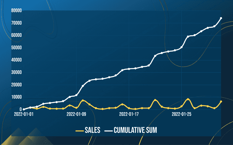
Below we show the final example which will calculate the cumulative sum and shows the output of our DataFrame and plot the results.
from pyspark.sql import SparkSession
from pyspark.sql import functions as F
from pyspark.sql.window import Window
from datetime import datetime
import matplotlib

spark = SparkSession.builder.appName("Aggregates").getOrCreate()

headers = ["date", "sales"]

data = [
    [datetime(2022, 1, 1), 100], [datetime(2022, 1, 2), 1543], [datetime(2022, 1, 3), 756],
    [datetime(2022, 1, 4), 2223], [datetime(2022, 1, 5), 765], [datetime(2022, 1, 6), 734],
    [datetime(2022, 1, 7), 762], [datetime(2022, 1, 8), 3422], [datetime(2022, 1, 9), 1500],
    [datetime(2022, 1, 10), 7332], [datetime(2022, 1, 11), 4200], [datetime(2022, 1, 12), 1121],
    [datetime(2022, 1, 13), 448], [datetime(2022, 1, 14), 1198], [datetime(2022, 1, 15), 1500],
    [datetime(2022, 1, 16), 4200], [datetime(2022, 1, 17), 1121], [datetime(2022, 1, 18), 448],
    [datetime(2022, 1, 19), 1198], [datetime(2022, 1, 20), 1198], [datetime(2022, 1, 21), 7653],
    [datetime(2022, 1, 22), 2345], [datetime(2022, 1, 23), 1246], [datetime(2022, 1, 24), 888],
    [datetime(2022, 1, 25), 2653], [datetime(2022, 1, 26), 8445], [datetime(2022, 1, 27), 1198],
    [datetime(2022, 1, 28), 3211], [datetime(2022, 1, 29), 2745], [datetime(2022, 1, 30), 1234],
    [datetime(2022, 1, 31), 6542],
]
df = (
    spark.createDataFrame(data, headers)
    .withColumn("cumsum", F.sum("sales").over(Window.orderBy("date")))
)
df.show(30)
We can quickly see an upward trend which indicates that all values are summed over time.
Moving average
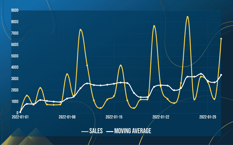
Another valuable calculation is the moving average. This calculation helps to determine the direction of a trend. It will filter out noise from random short-term fluctuations and smoothen data points, so longer-term cycles can be highlighted. Moving average requires a given set of values over a specific number of days in the past. In our example, we make use of 7 days in the past.
The window function we want to use is the avg function. It will calculate the average value over the specified window frame. The next step is to determine the window. We want to select all the values of the past 7 days, and order date in ascending order. In order to select the past 7 days, we have to make use of the FRAME clause. As we already described above, this is used to determine the lower and upper bounds of our frame.
In our example, we want to select the past 7 days based on the current row. We do this with a special statement, the rangeBetween clause. We have to set the lower and upper bound as input arguments. The lower bounds will be 7 days in the past, the upper bounds will be the current row. It is useful to know that when the upper bound is equal to the current row, we can simply skip the second argument.
So when we combine those elements, our final window will look something like this.
days = lambda i: i * 86400 # amount seconds in number of days

moving_7_day_window = (
	Window
	.orderBy(F.col("date").cast("timestamp").cast("long"))
	.rangeBetween(-days(7), Window.currentRow) # currentRow is not required
)
df.withColumn("mov_avg", F.avg("sales").over(moving_7_day_window))
There is a lot going on, so let me explain it in more detail.
The rangeBetween clause makes only use of integers or longs and it is not possible to use date or timestamp types. Therefore we have to cast our date column into a timestamp followed by a long type. Date types can not be directly cast as long types as they will be converted to null. Timestamps can be cast into long types which are actually converted to epoch seconds.
With the help of the days lambda function, we can easily calculate the total seconds based on the number of days. These seconds act as a lower bound that must be used in the rangeBetween clause. Important to use the minus seconds in the clause, otherwise the total seconds will be added based on the current row. Also, don’t forget to order the frame otherwise wrong rows will be selected.
We can easily call the F.avg over this window to calculate the moving average. The final example is shown below and it will output our DataFrame.
from pyspark.sql import functions as F
from pyspark.sql.window import Window
from pyspark.sql import SparkSession

spark = SparkSession.builder.appName("movingavg").getOrCreate()

headers = ["date", "sales"]

data = [
    ["2022-01-1", 100], ["2022-01-2", 1543], ["2022-01-3", 756],
    ["2022-01-4", 2223], ["2022-01-5", 765], ["2022-01-6", 734],
    ["2022-01-7", 762], ["2022-01-8", 3422], ["2022-01-9", 1500],
    ["2022-01-10", 7332], ["2022-01-11", 4200], ["2022-01-12", 1121],
    ["2022-01-13", 448], ["2022-01-14", 1198], ["2022-01-15", 1500],
    ["2022-01-16", 4200], ["2022-01-17", 1121], ["2022-01-18", 448],
    ["2022-01-19", 1198], ["2022-01-20", 1198], ["2022-01-21", 7653],
    ["2022-01-22", 2345], ["2022-01-23", 1246], ["2022-01-24", 888],
    ["2022-01-25", 2653], ["2022-01-26", 8445], ["2022-01-27", 1198],
    ["2022-01-28", 3211], ["2022-01-29", 2745], ["2022-01-30", 1234],
    ["2022-01-31", 6542],
]

days = lambda i: i * 86400

moving_7_day_window = ( Window.orderBy(F.col("date").cast("timestamp")
                    .cast("long")).rangeBetween(-days(7), Window.currentRow))

df = (
    spark.createDataFrame(data, headers)
    .select(
        # Change string date to date
        F.to_date(F.col("date")).alias("date"), F.col("sales"))
    .withColumn("mov_avg", F.avg("sales").over(moving_7_day_window))
)

df.show(30)
Next, we will show a new family of Functions that only exists in Window functions.
Ranking
The second category of window functions are Ranking functions. Ranking functions are used to assign a rank to each row within a partition of a result set. Depending on the function, ranking strategies can differ and some rows might receive the same value as other rows. Here are the most used Ranking window functions:
- ROW_NUMBER() assigns a sequential integer from the first row starting at 1
- RANK() ranks a value in a group of values based on the partition and order by
- DENSE_RANK() ranks a value in a group, but rows with equal values receive the same rank value
- NTILE() breaks values into a specified number of approximately equal size groups
- PERCENT_RANK() calculates the percent ranks a value in a group of values based on the partition and order by
Let’s start with an example that is widely used among data professionals.
Most recent records
Data comes from different source systems. One of these are OLTP systems, also known as Online Transaction Processing. Within these systems, entity states can change over time. E.g. the price of an item, or the shipment status of a product. When we load all these transactions into our system, we get multiple rows of the same entity. Usually, we only want to use the most recent record of an entity when we are performing certain calculations. We can easily select the most recent records with the help of a window function.
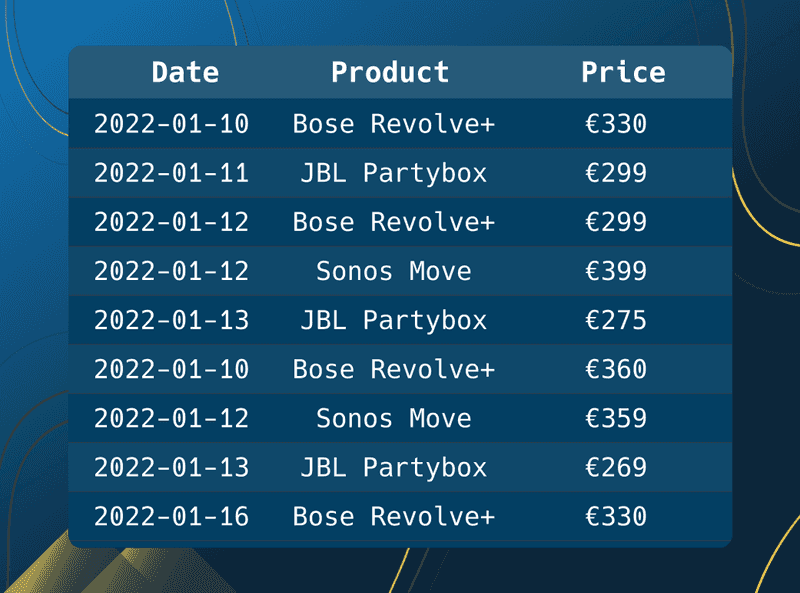
Let's start by preparing our dataset. For the two following examples, we make use of a product dataset. This dataset contains the price of an audio speaker on a particular date. We can see that the price fluctuates over time.
from pyspark.sql import functions as F
from pyspark.sql.window import Window
from datetime import datetime

headers = ["date", "product", "price"]

data = [
    [datetime(2022, 1, 10), "Bose Revolve+", 330],
    [datetime(2022, 1, 11), "JBL Partybox", 299],
    [datetime(2022, 1, 12), "Bose Revolve+", 299],
    [datetime(2022, 1, 12), "Sonos Move", 399],
    [datetime(2022, 1, 13), "JBL Partybox", 275],
    [datetime(2022, 2, 10), "Bose Revolve+", 360],
    [datetime(2022, 2, 12), "Sonos Move", 359],
    [datetime(2022, 2, 13), "JBL Partybox", 269],
    [datetime(2022, 2, 16), "Bose Revolve+", 330],
]
df = spark.createDataFrame(data, headers)

df.show()
# +-------------------+-------------+-----+
# |               date|      product|price|
# +-------------------+-------------+-----+
# |2022-01-10 00:00:00|Bose Revolve+|  330|
# |2022-01-11 00:00:00| JBL Partybox|  299|
# |2022-01-12 00:00:00|Bose Revolve+|  299|
# |2022-01-12 00:00:00|   Sonos Move|  399|
# |2022-01-13 00:00:00| JBL Partybox|  275|
# |2022-02-10 00:00:00|Bose Revolve+|  360|
# |2022-02-12 00:00:00|   Sonos Move|  359|
# |2022-02-13 00:00:00| JBL Partybox|  269|
# |2022-02-16 00:00:00|Bose Revolve+|  330|
# +-------------------+-------------+-----+
There is no window function that magically removes rows based on certain inputs, but we can do a trick that achieves this in two steps. We can make use of the row_number window function, which assigns a subsequent numbering to the rows in the window frame. If we order the frame on the date, but this time in descending order, we get the latest date on top of the frame. We then simply filter all the rows which have the value of row number one.
Because we want the most recent records of products and not all the rows, we have to use the partitionBy("product") clause. This will create different groups of product windows where the window function will be executed over. For every product group, a subsequent numbering is assigned.
Next, we will start adding subsequent numbering to our data in PySpark.
product_window = Window.partitionBy("product").orderBy(F.col("date").desc())

df = df.withColumn("row_num", F.row_number().over(product_window))
df.show()
# +-------------------+-------------+-----+-------+
# |               date|      product|price|row_num|
# +-------------------+-------------+-----+-------+
# |2022-02-16 00:00:00|Bose Revolve+|  330|      1|
# |2022-02-10 00:00:00|Bose Revolve+|  360|      2|
# |2022-01-12 00:00:00|Bose Revolve+|  299|      3|
# |2022-01-10 00:00:00|Bose Revolve+|  330|      4|
# |2022-02-13 00:00:00| JBL Partybox|  269|      1|
# |2022-01-13 00:00:00| JBL Partybox|  275|      2|
# |2022-01-11 00:00:00| JBL Partybox|  299|      3|
# |2022-02-12 00:00:00|   Sonos Move|  359|      1|
# |2022-01-12 00:00:00|   Sonos Move|  399|      2|
# +-------------------+-------------+-----+-------+
We can easily create a subsequent numbering with the F.row_number() function. Then we use a Window partitioned by the products and the date in descending order. A subsequent numbering is assigned to each row. The numbering restarts when a new product has been encountered.
The next step is to filter only the rows which have a value of row_num is one. We drop the row_num as it’s not necessary anymore.
recent_df = (
    df
		.filter(F.col("row_num") == 1)
    .drop("row_num")
)
recent_df.show()
# +-------------------+-------------+-----+
# |               date|      product|price|
# +-------------------+-------------+-----+
# |2022-02-16 00:00:00|Bose Revolve+|  330|
# |2022-02-13 00:00:00| JBL Partybox|  269|
# |2022-02-12 00:00:00|   Sonos Move|  359|
# +-------------------+-------------+-----+
If we would combine these steps into one script, we get something like this.
from pyspark.sql import functions as F
from pyspark.sql.window import Window
from datetime import datetime

headers = ["date", "product", "price"]

data = [
    [datetime(2022, 1, 10), "Bose Revolve+", 330],
    [datetime(2022, 1, 11), "JBL Partybox", 299],
    [datetime(2022, 1, 12), "Bose Revolve+", 299],
    [datetime(2022, 1, 12), "Sonos Move", 399],
    [datetime(2022, 1, 13), "JBL Partybox", 275],
    [datetime(2022, 2, 10), "Bose Revolve+", 360],
    [datetime(2022, 2, 12), "Sonos Move", 359],
    [datetime(2022, 2, 13), "JBL Partybox", 269],
    [datetime(2022, 2, 16), "Bose Revolve+", 330],
]

product_window = Window.partitionBy("product").orderBy(F.col("date").desc())

recent_df = (
    spark.createDataFrame(data, headers)
	.filter(F.col("row_num") == 1)
    .drop("row_num")
)
recent_df.show()
# +-------------------+-------------+-----+
# |               date|      product|price|
# +-------------------+-------------+-----+
# |2022-02-16 00:00:00|Bose Revolve+|  330|
# |2022-02-13 00:00:00| JBL Partybox|  269|
# |2022-02-12 00:00:00|   Sonos Move|  359|
# +-------------------+-------------+-----+
This is a very easy method of selecting the most recent records. This method works also great if you need to select the last values based on sequence numbers.
Break values into a specified number of approximately equal size buckets
Another thing we can do with ranking window functions is breaking up our dataset into specified approximately equal buckets. We achieve this with the use of the F.ntile function. It divides the ordered dataset into a number of buckets
In the following example, we use our audio speaker dataset where we want to create three equal-sized buckets based on the price of the speakers. We do this by calling the F.tile(3)which will try to equally divide three buckets based on the values in the Window. If the total size of the rows is not divisible by the total buckets, one of the buckets will contain one more entry.
Over this function, we need to use a Window partition by the product and order by the price in ascending order. We already demonstrated how to make such a window, so let’s show the code below.
.withColumn("bucket", F.ntile(3).over(Window.partitionBy("product").orderBy("price")))If we combine this Window Function with our current dataset, we have the following example.
from pyspark.sql import functions as F
from pyspark.sql.window import Window
from datetime import datetime

headers = ["date", "product", "price"]

data = [
    [datetime(2022, 1, 10), "Bose Revolve+", 330],
    [datetime(2022, 1, 11), "JBL Partybox", 299],
    [datetime(2022, 1, 12), "Bose Revolve+", 299],
    [datetime(2022, 1, 12), "Sonos Move", 399],
    [datetime(2022, 1, 13), "JBL Partybox", 275],
    [datetime(2022, 2, 10), "Bose Revolve+", 360],
    [datetime(2022, 2, 12), "Sonos Move", 359],
    [datetime(2022, 2, 13), "JBL Partybox", 269],
    [datetime(2022, 2, 16), "Bose Revolve+", 330],
]

product_window = Window.partitionBy("product").orderBy(F.col("date").desc())

bucket_df = spark.createDataFrame(data, headers).withColumn(
    "bucket", F.ntile(3).over(Window.partitionBy("product").orderBy("price"))
)
bucket_df.show()
# +-------------------+-------------+-----+------+
# |               date|      product|price|bucket|
# +-------------------+-------------+-----+------+
# |2022-01-12 00:00:00|Bose Revolve+|  299|     1|
# |2022-01-10 00:00:00|Bose Revolve+|  330|     1|
# |2022-02-16 00:00:00|Bose Revolve+|  330|     2|
# |2022-02-10 00:00:00|Bose Revolve+|  360|     3|
# |2022-02-13 00:00:00| JBL Partybox|  269|     1|
# |2022-01-13 00:00:00| JBL Partybox|  275|     2|
# |2022-01-11 00:00:00| JBL Partybox|  299|     3|
# |2022-02-12 00:00:00|   Sonos Move|  359|     1|
# |2022-01-12 00:00:00|   Sonos Move|  399|     2|
# +-------------------+-------------+-----+------+
We see that our price values are grouped into different buckets. Very useful if you want to rank the prices of your products.
Values
The last two examples belong to the values or analytical Window Functions. These functions are used to assign row values from other row values. This is especially useful to compare the current row with other rows. Let’s define most of the used functions.
- FIRST_VALUE() selects the first value of the first row in the window frame
- LAST_VALUE() selects the last value of the first row in the window frame
- LAG() selects the value for a row at a given offset prior to the current row in the window frame
- LEAD() selects the value for a row at a given offset following the current row in the window frame
- NTH_VALUE() selects the value of the specified row relative to the first row of the window frame
Using values of other rows is very powerful. Let's start with the first example.
Differences between the current row
One very valuable calculation is the determine the difference between the current row and the previous row. It can help us understand if there was an increase (positive difference) or a decrease (negative difference).
Let’s calculate the price difference for our audio speaker dataset.
We want to select the prior row based on the current row. We achieve this by using the F.lag Window Function. The argument of the F.lag is the column in which we want the value. The same window as in the earlier examples will be used.
window_spec = Window.partitionBy("product").orderBy("date")

lag_df = df.withColumn("previous_price", F.lag("price").over(window_spec))
lag_df.show()
# +-------------------+-------------+-----+--------------+
# |               date|      product|price|previous_price|
# +-------------------+-------------+-----+--------------+
# |2022-01-10 00:00:00|Bose Revolve+|  330|          null|
# |2022-01-12 00:00:00|Bose Revolve+|  299|           330|
# |2022-02-10 00:00:00|Bose Revolve+|  360|           299|
# |2022-02-16 00:00:00|Bose Revolve+|  330|           360|
# |2022-01-11 00:00:00| JBL Partybox|  299|          null|
# |2022-01-13 00:00:00| JBL Partybox|  275|           299|
# |2022-02-13 00:00:00| JBL Partybox|  269|           275|
# |2022-01-12 00:00:00|   Sonos Move|  399|          null|
# |2022-02-12 00:00:00|   Sonos Move|  359|           399|
# +-------------------+-------------+-----+--------------+
We see in the output that we do not have a previous price for every row. This is due to the fact that, depending on the current row and the window frame, no previous row was accessible.
We require a valid integer in order to calculate the difference between the rows. Otherwise, the calculation will also return a null value. As a result, we must filter out all null values. When all null values are removed, we calculate the difference by subtracting the price column from the previous_price column.
difference_df = (
	  df.filter(F.col("previous_price").isNotNull())
    .withColumn("difference", F.col("price") - F.col("previous_price"))
)
difference_df.show()
# +-------------------+-------------+-----+--------------+----------+
# |               date|      product|price|previous_price|difference|
# +-------------------+-------------+-----+--------------+----------+
# |2022-01-12 00:00:00|Bose Revolve+|  299|           330|       -31|
# |2022-02-10 00:00:00|Bose Revolve+|  360|           299|        61|
# |2022-02-16 00:00:00|Bose Revolve+|  330|           360|       -30|
# |2022-01-13 00:00:00| JBL Partybox|  275|           299|       -24|
# |2022-02-13 00:00:00| JBL Partybox|  269|           275|        -6|
# |2022-02-12 00:00:00|   Sonos Move|  359|           399|       -40|
# +-------------------+-------------+-----+--------------+----------+
Note, we have to keep in mind that the order is completely separate from the value we want to retrieve. If we put all the pieces together we have the following example.
from pyspark.sql import functions as F
from pyspark.sql.window import Window
from datetime import datetime

headers = ["date", "product", "price"]

data = [
    [datetime(2022, 1, 10), "Bose Revolve+", 330],
    [datetime(2022, 1, 11), "JBL Partybox", 299],
    [datetime(2022, 1, 12), "Bose Revolve+", 299],
    [datetime(2022, 1, 12), "Sonos Move", 399],
    [datetime(2022, 1, 13), "JBL Partybox", 275],
    [datetime(2022, 2, 10), "Bose Revolve+", 360],
    [datetime(2022, 2, 12), "Sonos Move", 359],
    [datetime(2022, 2, 13), "JBL Partybox", 269],
    [datetime(2022, 2, 16), "Bose Revolve+", 330],
]
df = spark.createDataFrame(data, headers)

window_spec = Window.partitionBy("product").orderBy("date")

difference_df = (
    df.withColumn("previous_price", F.lag("price").over(window_spec))
    .filter(F.col("previous_price").isNotNull())
    .withColumn("difference", F.col("price") - F.col("previous_price"))
)
difference_df.show()
# +-------------------+-------------+-----+--------------+----------+
# |               date|      product|price|previous_price|difference|
# +-------------------+-------------+-----+--------------+----------+
# |2022-01-12 00:00:00|Bose Revolve+|  299|           330|       -31|
# |2022-02-10 00:00:00|Bose Revolve+|  360|           299|        61|
# |2022-02-16 00:00:00|Bose Revolve+|  330|           360|       -30|
# |2022-01-13 00:00:00| JBL Partybox|  275|           299|       -24|
# |2022-02-13 00:00:00| JBL Partybox|  269|           275|        -6|
# |2022-02-12 00:00:00|   Sonos Move|  359|           399|       -40|
# +-------------------+-------------+-----+--------------+----------+
This example can also be used with following values based on the current row. We achieve this by simply swapping the F.lag with the F.lead window function.
First and last value of the month
For our last and final example, we will select the first and last value in a window frame from our dataset. This is useful to quickly compare the start and end values of the month.
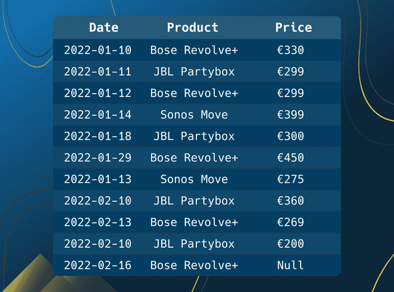
So let's start by augmenting our current radio speaker dataset to have more rows with dates in the future.
from pyspark.sql import functions as F
from pyspark.sql.window import Window
from datetime import datetime

headers = ["date", "product", "price"]

data = [
    [datetime(2022, 1, 10), "Bose Revolve+", 330],
    [datetime(2022, 1, 11), "JBL Partybox", 299],
    [datetime(2022, 1, 12), "Bose Revolve+", 299],
    [datetime(2022, 1, 14), "Bose Revolve+", 399],
    [datetime(2022, 1, 18), "JBL Partybox", 300],
    [datetime(2022, 1, 29), "Bose Revolve+", 450],
    [datetime(2022, 1, 13), "JBL Partybox", 275],
    [datetime(2022, 2, 10), "Bose Revolve+", 360],
    [datetime(2022, 2, 13), "JBL Partybox", 269],
    [datetime(2022, 2, 10), "Bose Revolve+", 200],
    [datetime(2022, 2, 16), "Bose Revolve+", None],
]
df = spark.createDataFrame(data, headers)
To simplify our dataset, we deleted a product and will add additional dates in the future. We also included a None value at the last available date for a speaker. We’ll cover later why we included a None value into our dataset as it showcases another powerful way of what you can do with the first and last Window Functions.
In our last example, we want to show the first and last value for a current year and month. We separate our date column into its own year and month columns.
.withColumn("year", F.year("date"))
.withColumn("month", F.month("date"))
The columns are then added to the Window Partition. Let’s define our Window.
window_spec = (
    Window.partitionBy("year", "month", "product")
    .orderBy("date")
    .rowsBetween(Window.unboundedPreceding, Window.unboundedFollowing)
)
We have defined a different FRAME clause. With rowsBetween you are able to select rows based on the number of rows from the current row. This is different from the rangeBetween clause as it uses a value range. If the row values are between that range all rows will be selected.
Window.unboundedPreceding is a special clause as it determines all the rows prior to the current row. With Window.unboundedFollowing we select all rows following the current row. We add the Window.unboundedPreceding clause as the first argument in the rowsBetween clause to set it as our lower bound.
Our Window Function will resemble this.
.withColumn("first_value", F.first("price", ignorenulls=True).over(window_spec))
.withColumn("last_value", F.last("price", ignorenulls=True).over(window_spec))
.show()
# +-------------------+-------------+-----+----+-----+-----------+----------+
# |               date|      product|price|year|month|first_value|last_value|
# +-------------------+-------------+-----+----+-----+-----------+----------+
# |2022-01-10 00:00:00|Bose Revolve+|  330|2022|    1|        330|       450|
# |2022-01-12 00:00:00|Bose Revolve+|  299|2022|    1|        330|       450|
# |2022-01-14 00:00:00|Bose Revolve+|  399|2022|    1|        330|       450|
# |2022-01-29 00:00:00|Bose Revolve+|  450|2022|    1|        330|       450|
# |2022-01-11 00:00:00| JBL Partybox|  299|2022|    1|        299|       300|
# |2022-01-13 00:00:00| JBL Partybox|  275|2022|    1|        299|       300|
# |2022-01-18 00:00:00| JBL Partybox|  300|2022|    1|        299|       300|
# |2022-02-10 00:00:00|Bose Revolve+|  360|2022|    2|        360|       200|
# |2022-02-10 00:00:00|Bose Revolve+|  200|2022|    2|        360|       200|
# |2022-02-16 00:00:00|Bose Revolve+| null|2022|    2|        360|       200|
# |2022-02-13 00:00:00| JBL Partybox|  269|2022|    2|        269|       269|
# +-------------------+-------------+-----+----+-----+-----------+----------+
The F.first and F.last Window Functions are used to choose the first and last values. It is critical that we provide an upper bound to the F.last function using Window.unboundedFollowing. Otherwise, the current row will be utilized as the last value. This will return incorrect values since values that belong later in the partition may exist.
Then we must select the year, month, product, first, and last values. Due to the number of rows, our result will contain duplicates. We can simply filter those out by using the distinct function. This will resemble the following.
.select(["year", "month", "product", "first_value", "last_value"])
.distinct()
# +----+-----+-------------+-----------+----------+
# |year|month|      product|first_value|last_value|
# +----+-----+-------------+-----------+----------+
# |2022|    1|Bose Revolve+|        330|       450|
# |2022|    1| JBL Partybox|        299|       300|
# |2022|    2|Bose Revolve+|        360|       200|
# |2022|    2| JBL Partybox|        269|       269|
# +----+-----+-------------+-----------+----------+
What you might not have noticed is that the last value of the Bose Revolve+ isn’t actually the last value. As we can see from our dataset, the last value is a None value. The first and last window functions are quite powerful since they allow you to pick values that are not null. We can simply accomplish this by using the *ignorenulls*=True argument to the Window Function. Our dataset shows that the lastest non-null value is 200.
If we combine all of the steps, our finished example will look like this.
from pyspark.sql import functions as F
from pyspark.sql.window import Window
from datetime import datetime

headers = ["date", "product", "price"]

data = [
    [datetime(2022, 1, 10), "Bose Revolve+", 330],
    [datetime(2022, 1, 11), "JBL Partybox", 299],
    [datetime(2022, 1, 12), "Bose Revolve+", 299],
    [datetime(2022, 1, 14), "Bose Revolve+", 399],
    [datetime(2022, 1, 18), "JBL Partybox", 300],
    [datetime(2022, 1, 29), "Bose Revolve+", 450],
    [datetime(2022, 1, 13), "JBL Partybox", 275],
    [datetime(2022, 2, 10), "Bose Revolve+", 360],
    [datetime(2022, 2, 13), "JBL Partybox", 269],
    [datetime(2022, 2, 10), "Bose Revolve+", 200],
    [datetime(2022, 2, 16), "Bose Revolve+", None],
]
df = spark.createDataFrame(data, headers)

window_spec = (
    Window.partitionBy("year", "month", "product")
    .orderBy("date")
    .rowsBetween(Window.unboundedPreceding, Window.unboundedFollowing)
)

first_last_df = (
    df.withColumn("year", F.year("date"))
    .withColumn("month", F.month("date"))
    .withColumn("first_value", F.first("price", ignorenulls=True).over(window_spec))
    .withColumn("last_value", F.last("price", ignorenulls=True).over(window_spec))
    .select(["year", "month", "product", "first_value", "last_value"])
    .distinct()
)
first_last_df.show()
# +----+-----+-------------+-----------+----------+
# |year|month|      product|first_value|last_value|
# +----+-----+-------------+-----------+----------+
# |2022|    1|Bose Revolve+|        330|       450|
# |2022|    1| JBL Partybox|        299|       300|
# |2022|    2|Bose Revolve+|        360|       200|
# |2022|    2| JBL Partybox|        269|       269|
# +----+-----+-------------+-----------+----------+
Conclusion
We covered a lot of ground in this comprehensive tutorial on Window Functions. We’ve seen that there are a variety of Window Functions that can perform complex calculations in PySpark. We run those functions across different partitions in our window. We’ve seen how crucial ordering is because it completely changes the outcome of our calculations. Finally, we cast a quick glance at the frame clause. By defining a rangeBetween and rowsBetween clause, we can easily include or exclude sets of rows within our partition. We select all the rows based on value ranges or the number of rows by specifying a lower and upper limit.
By utilizing these six Window Functions in PySpark, you power up your data processing and analysis. So don't wait any longer, start using window functions in your processing today!

